Lab 1 - with solutions

Please note that there is a file on Canvas called Getting started with R which may be of some use. This provides details of setting up R and Rstudio on your own computer as well as providing an overview of inputting and importing various data files into R. This should mainly serve as a reminder.

Recall that we can clear the environment using rm(list=ls()) It is advisable to do this before attempting new questions if confusion may arise with variable names etc.

Example 1

This example will provide the full details of the confidence interval example we met in the lectures. We will create a confidence interval for the variable StudentAge in the Student Age dataset. Please follow the steps below:

Firstly, we input the dataset into R, attach it and check it using the “head” command (recall that this provides the first 6 entries).

library(foreign)
Student <- read.spss("Student Age.sav", to.data.frame=T)

Or, if you prefer to search for the dataset file, use:

Student <- read.spss(file.choose(), to.data.frame=T)

attach(Student)
head(Student)

  StudentAge
1         55
2         60
3         58
4         20
5         22
6         59

In order to determine the correct method, we test the normality of the data. We first do this visually - we first consider a basic histogram:

hist(StudentAge)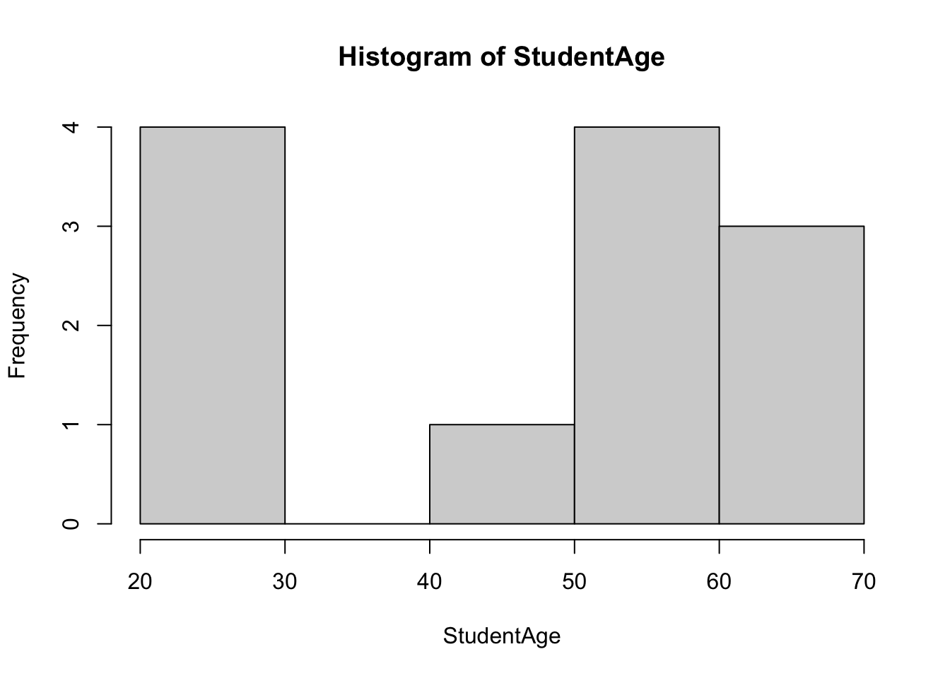

The code below produces a histogram with an overlaid probability density function. Make sure you understand the code and the output generated.

hist(StudentAge, prob=T, breaks=seq(from=0,to=100, by=10), xlab="Student Age", 
     main="Histogram of Student Age", las=1)
lines(density(StudentAge),col=2)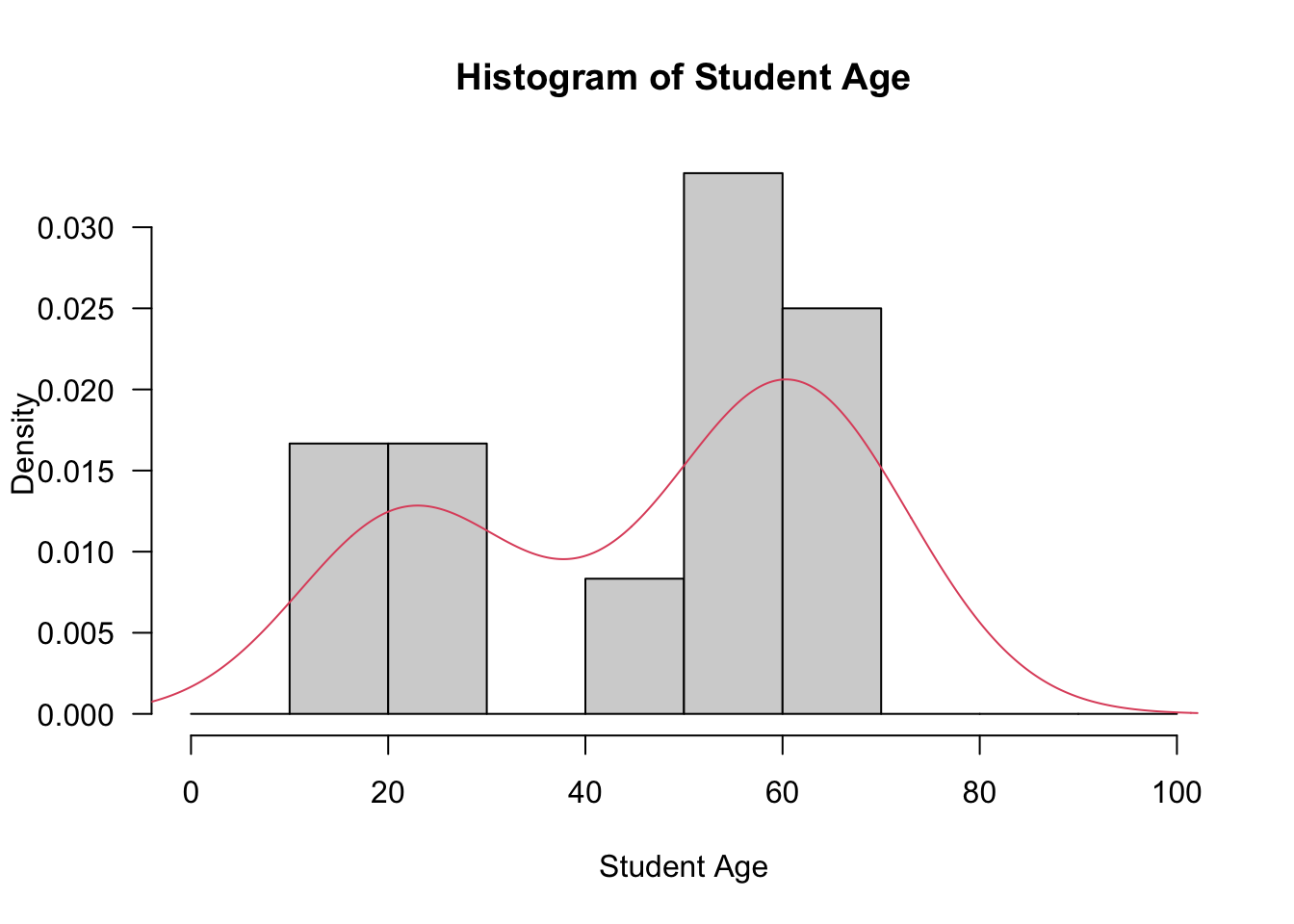

Next we perform the Shapiro-Wilk test and the Kolmogorov-Smirnov test (with Lilliefors’ correction). Note that we require the “nortest” package to use Lilliefors’ test.

shapiro.test(StudentAge)


    Shapiro-Wilk normality test

data:  StudentAge
W = 0.83438, p-value = 0.02367

install.packages("nortest")

library(nortest)
lillie.test(StudentAge)


    Lilliefors (Kolmogorov-Smirnov) normality test

data:  StudentAge
D = 0.25006, p-value = 0.03682

You should have come to the conclusion the the variable StudentAge is not normally distributed. Therefore, we cannot use traditional parametric techniques to produce confidence intervals (as seen in MA-192) and hence we use the bootstrap method. The code below is used to calculate the mean of each bootstrap sample and m.mean is just the name of the function to calculate the mean of each bootstrap sample with index i. We use the standard 1000 resamples. Note that we must use the boot package.

library(boot)
my.mean <- function(x, i){return( mean( x[i] ) )}
age.boot <- boot(Student$StudentAge, my.mean, 1000)

The code below is then used to produce bootstrap confidence intervals. Note the options, e.g. changing the significance level and specifying the type of bootstrap C.I. All three types of bootstrap confidence interval seen in the lectures are included below.

boot.ci(age.boot, conf=0.95, type=c("perc", "bca", "norm"))

BOOTSTRAP CONFIDENCE INTERVAL CALCULATIONS
Based on 1000 bootstrap replicates

CALL : 
boot.ci(boot.out = age.boot, conf = 0.95, type = c("perc", "bca", 
    "norm"))

Intervals : 
Level      Normal             Percentile            BCa          
95%   (35.92, 57.35 )   (35.83, 56.91 )   (35.00, 56.17 )  
Calculations and Intervals on Original Scale

You should obtain an output similar to the one above in your Console, noting that bootstrapping is a random process so the actual intervals will vary.

Exercise 1

Create a 95% confidence interval for the BMI variable in the BMI Scores dataset. Firstly, test the normality of the data, and if a bootstrap confidence interval is required create both percentile and BCa bootstrap confidence intervals for the mean of BMI.

Hint: The dataset needs to be made R friendly and you need to think about how to import it into R. One way is to save it as a csv file and use the code: BMIScores<-read.csv(file.choose(), header=T)

Solution

Note that this dataset will need to be “tidied” first.

BMIScores <- read.csv(file.choose(), header=T)

head(BMIScores)

  Patient BMI
1       1  32
2       2  29
3       3  33
4       4  15
5       5  16
6       6  16

attach(BMIScores)

We now visualise the data.

hist(BMI, prob=T, breaks=seq(from=0,to=100, by=10), xlab="BMI", main="Histogram of BMI Scores", las=1)
lines(density(BMI),col=2)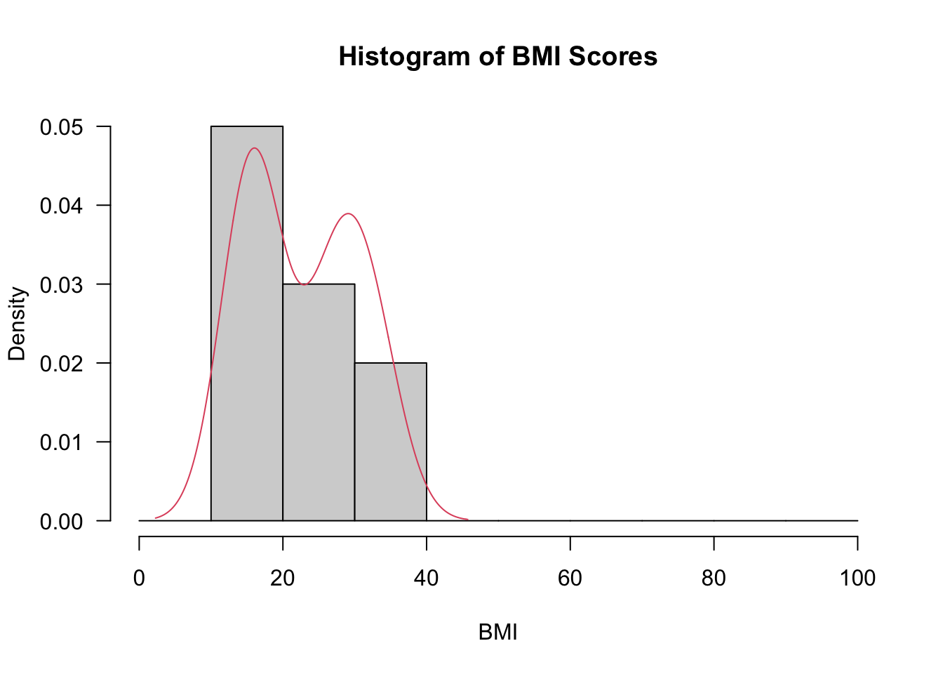

Next we perform tests of normality.

shapiro.test(BMI)


    Shapiro-Wilk normality test

data:  BMI
W = 0.82976, p-value = 0.03324

install.packages("nortest")

library(nortest)
lillie.test(BMI)


    Lilliefors (Kolmogorov-Smirnov) normality test

data:  BMI
D = 0.27323, p-value = 0.03303

The output of the tests of normality above indicate that we should consider bootstrap confidence intervals

library(boot)
my.mean <- function(x, i){return( mean( x[i] ) )}
BMI.boot <- boot(BMI, my.mean, 10000)
boot.ci(BMI.boot, conf=0.95, type=c("perc", "bca", "norm"))

BOOTSTRAP CONFIDENCE INTERVAL CALCULATIONS
Based on 10000 bootstrap replicates

CALL : 
boot.ci(boot.out = BMI.boot, conf = 0.95, type = c("perc", "bca", 
    "norm"))

Intervals : 
Level      Normal             Percentile            BCa          
95%   (18.16, 27.00 )   (18.30, 27.10 )   (18.30, 27.10 )  
Calculations and Intervals on Original Scale

Exercise 2

Why would we not perform a bootstrap confidence interval on the variable Heightincm in the dataset MA-777 Student Height? Give the standard confidence interval for the mean of student height (use the code t.test("variable name", conf.level=0.95), as used in MA-192).

Hint: Another way to import Excel files into R is using the Import Dataset option.

Solution

The dataset is currently an xlsx file, therefore use either method to import this file. I have used the “Import Dataset” feature.

attach(MA_777_Student_Height_1)

The following object is masked _by_ .GlobalEnv:

    Student

In the histogram below I adjust the breaks to make the histogram more presentable

hist(`Height in cm`, prob=T, breaks=seq(from=100,to=200, by=10), xlab="Height", main="Histogram of MA-777 Student Height", las=1)
lines(density(`Height in cm`),col=2)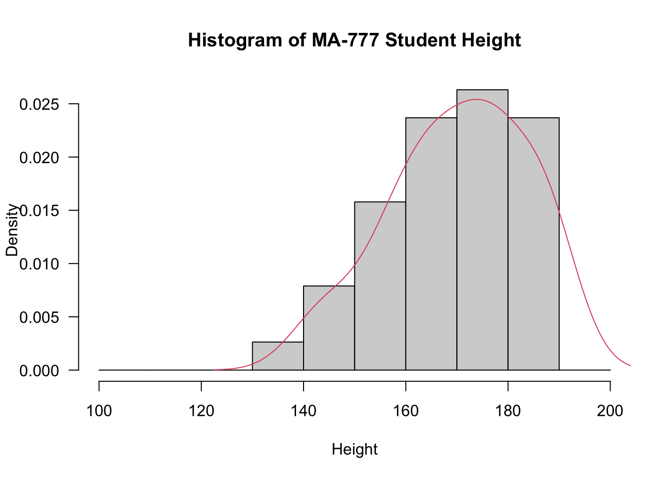

Now we perform tests of normality

shapiro.test(`Height in cm`)


    Shapiro-Wilk normality test

data:  Height in cm
W = 0.9614, p-value = 0.2107

lillie.test(`Height in cm`)


    Lilliefors (Kolmogorov-Smirnov) normality test

data:  Height in cm
D = 0.084389, p-value = 0.7082

The visualistaions and tests above indicate that the data are normally distributed, therefore we do not use bootstrap methods. Instead we use standard techniques for confidence intervals, see below. The default option to create confidence intervals in R is the t confidence interval.There are a number of ways of doing this including t.test in the package Rmisc.

t.test(`Height in cm`, conf.level=0.95)


    One Sample t-test

data:  Height in cm
t = 77.869, df = 37, p-value < 2.2e-16
alternative hypothesis: true mean is not equal to 0
95 percent confidence interval:
 165.8841 174.7475
sample estimates:
mean of x 
 170.3158

Example 2

In this example we will investigate skewness of the variable Salary in the Salary (Skewness) dataset. Follow the steps below:

Firstly, import the SPSS dataset into R and check the first 6 entries:

SalaryData <- read.spss(file.choose(), to.data.frame=T)

SalaryData <- read.spss("Salary (Skewness).sav", to.data.frame=T)
attach(SalaryData)
head(SalaryData)

One option to investigate skewness is to produce a histogram, but we should first take a look at the data to get a better idea of the range of values and what “breaks” we should use, see below:

SalaryData

hist(Salary, prob=F, breaks=seq(from=2000,to=100000, by=9000),
     xlab="Salary", main="Histogram of Salary Data", las=1)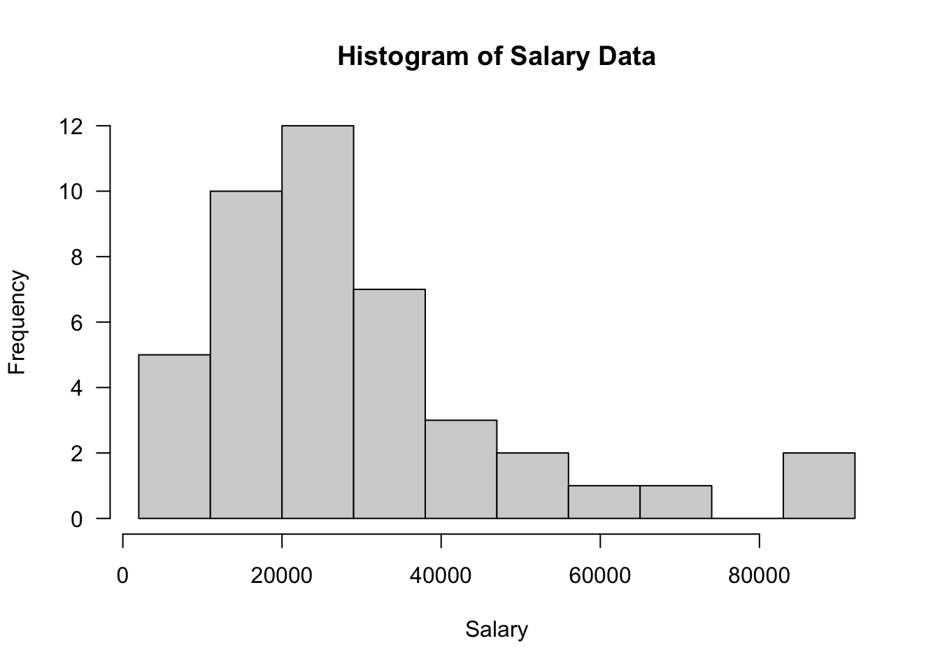

You should obtain the above output, indicating left-skewed data.

Next we calculate the skewness statistic, for which we require the moments package.

install.packages("moments")

library(moments)
skewness(Salary)

[1] 1.515277

You should obtain the value 1.515 (to 3dp), as per the output above, providing further evidence of skewness (since the skewness statistic is \(>1\)).

Exercise 3

The Student Current Account Balance dataset contains the current account balance of 18 students at the end of term. Check the skewness of the variable Balance. Why is a bootstrap confidence interval appropriate in this case? Find a 95% BCa bootstrap confidence interval for the mean of Balance.

Hint: note that the sample size is small. Skewness of data suggests it is not normally distributed, but this can be double-checked using the usual tests.

Solution

We first import the data.

CurrentAccount <- read.spss(file.choose(), to.data.frame=T)

attach(CurrentAccount)
head(CurrentAccount)

We now check the skewness and perform tests of normality on the variable Balance

skewness(Balance)

[1] 1.082313

shapiro.test(Balance)


    Shapiro-Wilk normality test

data:  Balance
W = 0.89573, p-value = 0.04845

library(nortest)
lillie.test(Balance)


    Lilliefors (Kolmogorov-Smirnov) normality test

data:  Balance
D = 0.20631, p-value = 0.04142

A histogram may also help:

hist(Balance, prob=T, breaks=seq(from=-300,to=400, by=50), xlab="Balance", main="Histogram of Current Account Balance", las=1)
lines(density(Balance),col=2)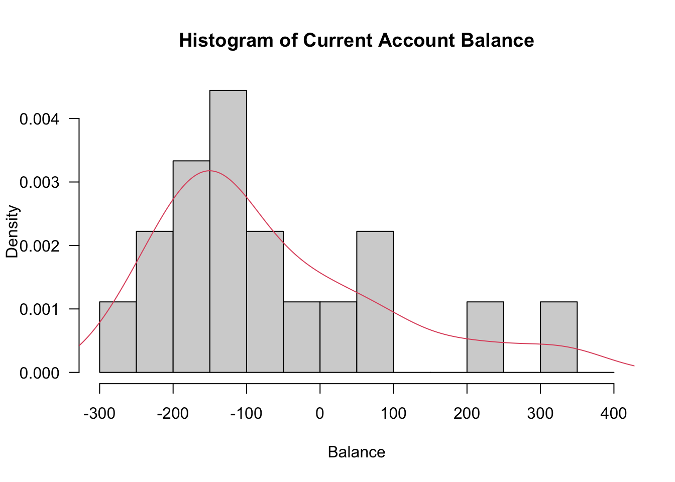

Balance

 [1] -154 -240  -10    5 -127 -140  100  -55 -143 -132  -80 -165   67 -182 -215
[16]  210 -253  330

Since the data does not seem to be normally distributed we perform a bootstrap confidence interval (BCa) as requested in the question.

library(boot)
my.mean <- function(x, i){return( mean( x[i] ) )}
Balance.boot <- boot(Balance, my.mean, 10000)
boot.ci(Balance.boot, conf=0.95, type=c("bca"))

BOOTSTRAP CONFIDENCE INTERVAL CALCULATIONS
Based on 10000 bootstrap replicates

CALL : 
boot.ci(boot.out = Balance.boot, conf = 0.95, type = c("bca"))

Intervals : 
Level       BCa          
95%   (-125.23,   20.17 )  
Calculations and Intervals on Original Scale